How to Lock Formulas in Excel? Protect formula in Excel? Confused? Here is the blog to know how to lock excel formulas.
Imagine Your boss wants you to protect a workbook, but she also wants to be able to change a few cells after you are done. So, before you password protected the workbook (or a worksheet), you unlocked some cells. Now that your boss is done, you can lock the cells.
Think Is it possible for you to protect your particular cells contain formulas?
The answer is Yes!
The most common way of preventing people from tampering with your Excel formulas is to Protect the worksheet.
Excel Vlookup formula – Guidebook
Bored of downloading text heavy / copy-pasted eBooks?
If Yes, you will enjoy this guidebook on ‘Excel Vlookup Formulas’ – VLOOKUP, HLOOKUP, MATCH & INDEX.
How to Lock Formulas in Excel (Step By Step Guide)
Here are the steps to lock formulas in Excel (explained in detail later on):
Step 1: Select the cell with formulas that you want to lock & Press Ctrl + 1
Step 2: In the format cells dialog box, select the protection tab.
Step 3: Check the “Locked” Option in Excel
Step 4: Click Ok & Apply
Let see how to lock formulas in Excel by following steps!
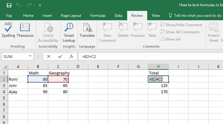
Step 1: Create a table the same as the above picture. This table is showing students’ marks of two subjects Maths and Geography. In the cells of column H, we have used a formula that calculates the total marks of each student in these two subjects. Say, in cell H2 we have used the formula given below:
=B2+C2
We are going to lock only those formulas in column H.
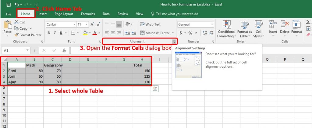
Step 2: Here we have two objectives to lock only formulas. Firstly, we have to unlock the whole cells of the worksheet,. Secondly, we will protect only formulas. So now Select the whole table as like the above picture. Now click the Home tab and in the Alignment group, choose the small arrow to open the Format Cells dialog box.
Step 3: On the Protection tab, Unchecked the Locked check box, and then click OK.
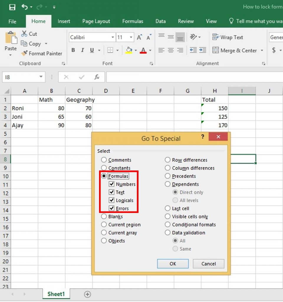
Step 4: Go to the Home tab. From the Editing group, click Find & Select button and choose Go To Special.
15Excel Data Cleaning Tricks Guidebook
Bored of downloading text heavy / copy-pasted eBooks? If Yes, you will enjoy this guidebook (43 pages)
Step 5: In the Go To Special dialog box, check the Formulas radio button. This will select the checkboxes for all formula types. Now click OK.
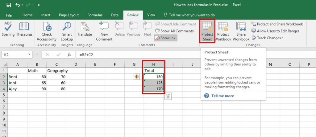
Step 6: Now it has selected only those cells to contain a formula. Now locked again only this selected formula from Format Cells dialog box following previous steps. Now on the Review tab in the ribbon select Protect Sheet from Changes group.
Step 7: The Protect Sheet dialog window will appear. Check “Select locked Cell” and “Select Unlocked Cell”. Now click OK.
Tips: In the Protect Sheet dialog window You can use a password in the text box named “Password to unprotect sheet”. In this way when someone will try to unprotect this, it will not be possible for him to unprotect without your given password. Only you can Unprotect or Unlock this formula. So, be careful and remember your given password to unprotect this formula.
Step 8: Click on any cell of column H that contains a formula, It will show a message like the above picture. But You can edit another cell. This is the simple way you can hide and lock particular cells that contain formulas in Excel.
Tips: When you want to unprotect it again, just simply select the Review tab, then click the Unprotect Sheet and use your given password. Then it will be unprotected again for you. If you want to learn more about Excel Tips & Tricks. Please check our latest Excel Ninja Course that offers high-quality videos with lifetime access.
Now We have successfully locked our formulas in Excel!
15 Pivot Tables Tricks for Pros
15 Pivot Table tricks to make your Excel data analysis smarter! 5,600+ downloads.