Wrap Text is the most known function of excel. There are times when it is difficult to adjust long texts within an excel cell. When you’ve much text piled up and it should be present in the spreadsheets. Or if you have failed to fit your text in an Excel Cell. Excel Wrap Text option will help you fit a long text in an excel cell or adjust long texts within an excel cell.
Excel is one of the best data analysis tools, that one can learn before starting their first Data Analysis Project. Therefore it’s the best time to learn Excel and become certified in Excel Master Program.
Well, what you can do about this is, learn how to make an excel cell expand to fit the text.
Shortcut to Wrap Text in Excel is: Alt + Enter
(Press and hold the Alt key and then press and release the Enter Key without releasing the Alt key on the Keyboard.)
Excel Vlookup formula – Guidebook

Bored of downloading text heavy / copy-pasted eBooks?
If Yes, you will enjoy this guidebook on ‘Excel Vlookup Formulas’ – VLOOKUP, HLOOKUP, MATCH & INDEX.
What are the steps to Wrap Text Cells in Excel?
To wrap text in Excel Cells you have to follow the below Steps,
- Go to Home Tab, go to Alignment Group
- Click on the Wrap Text Button
- Press Ctrl + 1
- Click on the selected cells
- Click on the Format Cells dialog box
- Go to Alignment Tab
- Check/Tick on the Wrap Text Checkbox
- Click OK.
When you want to fit long text in Excel using Wrap Text, Microsoft lets you do this by offering a few other ways. The tutorial is all about the Microsoft Excel Wrap Text Feature and also about the quick tips on how to use Wrap Text in Excel wisely.
Interested to learn ‘How to freeze Rows and Columns in Excel? Click on the link and check now. CLICK
When do you use wrap text?
Sometimes, there is a large amount of Data in an Excel Cell and you don’t know how to fit the long text in an Excel Cell. The reason is, that the data is too large. During this situation, the two situations are for sure to strike.
- When the columns on the right side are empty, you’ll observe that the cell border of the Columns will be extended with long text strings.
- When there is any data in the adjacent cell at the right. At the cell border, you’ll observe the text string is cut off.
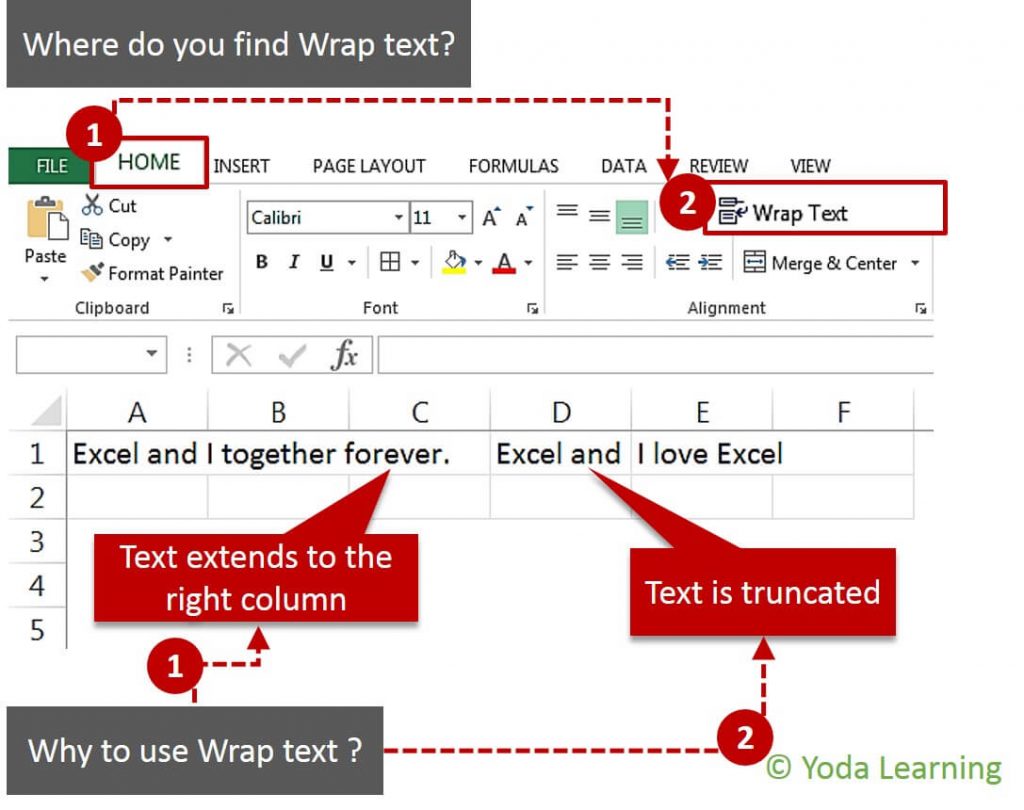
In the image, you’ll get to see where to find the Excel Wrap Text icon in Excel.
Also, you’ll find those two cases are displayed:
- The longer text is extending to the right column
- The longer text is getting shortened.
Do you know how to use the Excel Wrap Text Feature? The Excel Wrap Text Feature will help you to display and learn how to fit the long text in Excel using Wrap Text in an individual cell. What happens is, that there are times when some texts get lost in the next line. The main advantage is, that the text here won’t overflow in the adjacent cell.
With “Wrapping Text” you’re able to wrap the text in Multiple Lines rather than displaying it on one long line. This helps you in avoiding the “Truncated Column effect”. As you can see, the text is overflowing from the Column and getting Truncated towards the right. Which is making the readability of the text a lot easier than before. Also, it makes text adjustments for its printing.
Add on: The main contribution of the Wrap text feature in Excel is that, it helps to retain the main width of the Column in the entire Worksheet.
How to wrap text automatically?
If you wish to obtain the lengthy text string or see it on Multiple Lines or lines of text in a cell, you need to select the cell(s) that you wish to Format. Now, you need to turn on the Excel Text Wrap Feature.
Steps to Wrap Text Automatically using the Wrap Text button:
- Select the cells
- Go to the Home Tab
- Click the Wrap Text Button

Excel Vlookup formula – Guidebook
Bored of downloading text heavy / copy-pasted eBooks?
If Yes, you will enjoy this guidebook on ‘Excel Vlookup Formulas’ – VLOOKUP, HLOOKUP, MATCH & INDEX.
Or you can:
- Select the cells
- Press Ctrl + 1, to open the Format Cells dialog box
- Check/Tick the Wrap Text Checkbox and then click OK

Compared to the first method, this will be a tricky and complicated one. It might need a few of your Extra clicks but with this wrapping, the text would become easy.
Cell Formatting: Here will bargain for you sometime. If you wish to bring changes in the Cell Formatting at a time, the wrap-up text option will be one change.
Important Tip: When you observe that the Wrap Text Checkbox is Solid-filled. This indicates that setting the selected Cells has a different Text Wrap.
Result: It doesn’t matter what method you’re using. The data in the selected cells wraps to fit the column width. This is why, on changing the column width, text wrapping will adjust automatically.
How to unwrap text in Excel?
Click on the Wrap Text Button (In the Home Tab> alignment group)
There are two ways to Unwrap Text in Excel:
Method 1: Clear the text checkbox on the Alignment tab
Method 2: Press Ctrl+1. This will open the Format Cells Dialog box
Steps for Method 1:
- Select the Cells
- Go to the Home Tab
- Go to Wrap Text and Unselect the Wrap Text Option
Steps for Method 2:
- Select the Cells
- Press Ctrl+1. This opens the Format Cells Dialog box
- In the Alignment group, Clear/untick/uncheck the Wrap text checkbox

How to insert a line break manually?
When inserting a line break manually, these steps are to be followed:
- Click on any of the Cell Press F2 and enter the cell edit mode
- Press Alt+Enter (Place the cursor where you want to break the line)
How to autofit Fixed row height in Excel?
In case, if all the wrapped texts are visible in a cell, the certainty is, that the row might be set to a particular height. There are two methods by which you can fix this Problem:
First Method: Set a specific height for the row, this can be done by clicking on the Row Height
Second Method: Autofit the height for the Row by selecting the Autofit Row Height Option.
Method 1:
- Select the Problematic cells
- Go to the Home Tab
- In the cells group, Click on Format
- Select/Click on the Row-height Option
- In the Row Height Dialog Box, Enter the Row-height you want (In our case, we have taken 45.)
Method 2:
- Select the Problematic cells
- Go to the Home Tab
- In the cells group, Click on Format
- Select/Tick on the Auto-fit Row Height Option
Method 1 & Method 2 Explain in below Image

How to Merge and center in Excel?
If you have merged Cells, wrap text won’t work.
To Wrap the Text of Merged cells, you’ll have to:
- Unmerge the cells by going to Home Tab> Alignment Group> Merge & Center dropdown> Click on the Unmerge Cells
- Select the Unmerged Cells
- Click on Wrap Text
Suppose, if your cell doesn’t show Wrap Text then you’ll need to adjust the Row Height.
Also, the Steps to adjust the Row Height are explained above.
Excel’s Wrap Text feature isn’t flexible when working with the merged cells. So, you must decide which feature will work best for the particular Worksheet. Using the merge Cells Option, you’ll be able to display the whole text string in the columns. You’ll need to make the Column Wider.
You’ll observe the cell here is wide enough for displaying the value.
Do not wrap a cell(s) that is already wide enough to display its contents. The reason is, that if you try to, nothing will happen to the text. In case, if you resize the Column for further entries, the column might become too narrow in size. It becomes difficult to adjust the longer entries in this. Toggle the Excel Wrap Text Button off and then on again, just in case, if you wish to fit a long text in Excel using wrap text.
Conclusion

When you insert a line break it turns on the Wrap Text Option automatically. Whereas when you enter the line break manually, this will stick at the same place even when the Column is made wider.
When you turn off the Text Wrapping, the data will be displayed in one line in a cell. Also, If you wish to see the line breaks inserted, you’ll be able to find these in the Formula Bar. You can learn more tricks of excel in our online advanced excel course.
In the image, you’ll be able to observe both situations. A-Line break is entered after the word ‘love”.
15 Pivot Tables Tricks for Pros
15 Pivot Table tricks to make your Excel data analysis smarter! 5,600+ downloads.
Most Popular Tricks are #3, #7 & #12