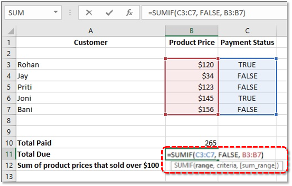
The SUMIF function is a built-in function in Excel that is categorized as a Math/Trig Function. It can be used as a worksheet function (WS) in Excel. As a worksheet function, the SUMIF function can be entered as part of a formula in a cell of a worksheet. You can try the SUMIF function to add numbers in a range based on multiple criteria.
To learn how to use SUMIF, we also have to know what is SUMIF and when can we use it?
Excel Vlookup formula – Guidebook

Bored of downloading text heavy / copy-pasted eBooks?
If Yes, you will enjoy this guidebook on ‘Excel Vlookup Formulas’ – VLOOKUP, HLOOKUP, MATCH & INDEX.
What is the SUMIF Function?
The Excel SUMIF function finds the values in a supplied array, that satisfy given criteria, and returns the sum of the corresponding values in a second supplied array.
When to use SUMIF?
SUMIF Function is used to add the specified cells based on the single or multiple supplied criteria. Sometimes we require conditional sum in Excel then we can use this function to add all numbers in a particular given range. SUMIF function is based on the three parameters- range, criteria, and sum_range. Every parameter has its own functionality and also depends on SUMIF multiple criteria.
Function Syntax
The SUMIF Function in Excel has the following syntax:
=SUMIF(range, criteria, sum_range)
Parameters
range: The range of cells that you want to apply the criteria against.
criteria: The criteria used to determine which cells to add.
sum_range: Optional. It is the range of cells to sum together. If this parameter is omitted, it uses range as the sum_range.
Now, let see how to use SUMIF to excel with a Case Study.

Case Study: Consider that we have a shop and 5 people have ordered goods from us. Some people have paid us, but some haven’t. We want to calculate how much in total has been paid to us and how much is still owed.
Excel Vlookup formula – Guidebook

Bored of downloading text heavy / copy-pasted eBooks?
If Yes, you will enjoy this guidebook on ‘Excel Vlookup Formulas’ – VLOOKUP, HLOOKUP, MATCH & INDEX.
We can do it using SUMIF
Let’s go through the following steps.
Step 1: Open Excel sheet and from Row 1, create three columns named Customer, Product Price and Payment Status. Enter data under these 3 columns as shown in the above picture. Here we will calculate:
- Total Paid Price (Cell A10)
- Total Due Price (Cell A11)
- Sum of product prices that sold over $100 (Cell A12)

In cells B10, B11, and B12, we’ll use a SumIF function to work out Total Paid Price, Total Due Price, and Sum of product prices that sold over $100. Here’s the SumIF function again:
=SUMIF(range, criteria, sum_range)
Calculate Total Paid Price
The range of cells that we want to check is True and False values in the C column. The criteria is whether they have paid (True) and the Sum_Range is what we want to add up (in Column B).
Step 2: In cell B10, enter the following formula:
=SUMIF(C3:C7, TRUE, B3:B7)
Step 3: Press Enter. Excel should give you the answer 265 in cell B10. In the formula, we told SumIF to first check the values in the cells C3 to C7(range). Then we said look for a value of TRUE (criteria). So we wanted the values in the B column adding up if a criterion of TRUE was indeed found (sum_range). Finally, we got the result 265 that has been paid in total.

Calculate Total Due Price
15 Excel Data Cleaning Tricks Guidebook
Bored of downloading text heavy / copy-pasted eBooks? If Yes, you will enjoy this guidebook (43 pages)
Step 4: In cell B11, enter the following formula:
=SUMIF(C3:C7, FALSE, B3:B7)

Step 5: Press ENTER. Excel should give you the answer 313 in cell B11. In the formula, we told SumIF to first check the values in the cells C3 to C7 (range). Then we said look for a value of FALSE (criteria). So we wanted the values in the B column adding up if a criterion of FALSE was indeed found (sum_range). Finally, we got the result 313 is Total Due Price.

Calculate the Sum of product prices that sold over $100
Step 6: In cell B12, enter the following formula:
=SUMIF(B3:B7,”>100″)

Step 7: Press ENTER. Excel should give you the answer 544 in cell B12. In the formula, we told SumIF to first check the values in the cells B3 to B7 (range). Then we said look for a Price value higher than $100. So we wanted the values in the B column adding up if a criterion of >100 was indeed found (sum_range). Finally, we got the result 544 is Sum of product prices that sold over $100.
Tips: There are many ways to find out a particular Sum. Say, if you want to calculate the total price sold out to a particular customer named Joni, then just shift your range of that formula from B3:B7 to A3:A7 and type criteria like the name of customer Joni then select the sum_range B3:B7. So, the formula would be:
=SUMIF(A3:A7, “Joni”, B3:B7)
Now You have successfully learned how to use SUMIF Formula in Excel
15 Pivot Tables Tricks for Pros
15 Pivot Table tricks to make your Excel data analysis smarter! 5,600+ downloads.
Most Popular Tricks are #3, #7 & #12

