Comparing values in Excel is something that we all do once in a while. Microsoft Excel offers a number of options to compare and match data, but most of them focus on searching in one column. When using Excel for data analysis, accuracy is the most vital concern. Incorrect information may lead to missed deadlines, misjudged trends, wrong decisions, and lost revenues. While Excel formulas are always perfectly true, their results may be wrong because some flawed data penetrated into the system.
Excel Vlookup formula – Guidebook

Bored of downloading text heavy / copy-pasted eBooks?
If Yes, you will enjoy this guidebook on ‘Excel Vlookup Formulas’ – VLOOKUP, HLOOKUP, MATCH & INDEX.
In this case, the only remedy is to check data for accuracy. It’s no big deal to compare two cells manually, but it’s next to impossible to spot the differences between hundreds and thousands of text strings. In this tutorial, we will learn how to compare values in Excel and find matches and differences between them.
Now, let’s go through the following steps to compare the values of two cells.
Case Study 1: Case-sensitive formula to compare values in Excel.

Imagine that sometimes it may be important for you not only to compare text in two cells but also to compare the character case. Case-sensitive text comparison can be done using the Excel EXACT function
Learn compare values in Excel by following steps:-
So here are the steps that you have to follow to compare values in excel from 2 columns:
- Step 1: First Select the Entire dataset where you compare the values
- Step 2: Click on Home Tab in Excel
- Step 3: Go to Style Group, click on “Conditional Formatting” Option
- Step 4: Move your cursor on the Highlight Cell Rules Option
- Step 5: Click On Duplicate Values in Excel Cell
- Step 6: In Duplicate Values Dialog Box, select ‘Duplicate’
- Step 7: Click the format button & specify the format, where you want to compare the values in excel
- Step 8: Click OK & you will get compared Values in Excel
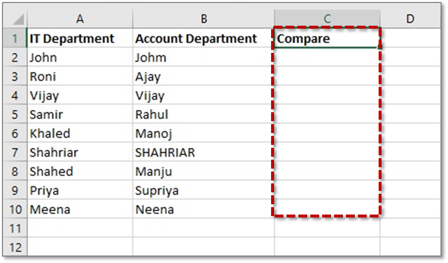
Step 1: Create a table the same as the above picture. This table is showing the list of Two departments of an office. We will compare two cells between each row with a case-sensitive formula. Column C will show the exact matching of each cell. If the exact match found, then the result will be TRUE, if not then the result will be FALSE.

Step 2: Now input this formula in cell C2 to compare cell A2 and B2:
- =EXACT(A2, B2)
- Now press ENTER.

Now, cell C2 is showing False because John and Johm do not match exactly.

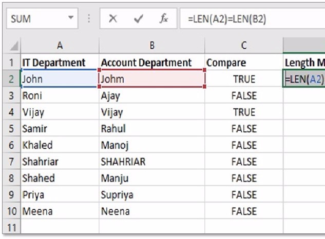
Step 3: Copy the formula into another cell of column C. Now we will get the above result like the picture. Here we can see only row 4 has the TRUE result. Means cell A4 and B4 contain the exact value Vijay, this is the reason we have got the result TRUE.
Tip 1: If you want to see Exact instead of TRUE as result and Not Exact instead of FALSE, you can use this formula instead of our previous formula and see the magic:
- =IF(EXACT(A2 ,B2), “Exactly equal”, “Not equal”)
So, in this way, we can compare two cells value with Case-sensitive formula!
Excel Vlookup formula – Guidebook

Bored of downloading text heavy / copy-pasted eBooks?
If Yes, you will enjoy this guidebook on ‘Excel Vlookup Formulas’ – VLOOKUP, HLOOKUP, MATCH & INDEX.
Case Study 2: Compare values in Excel by string length.

Sometimes we want to check if the text strings in each row contain an equal number of characters.
How can we check text strings in each row contain an equal number of characters?
Easy, first, you get the string length of two cells using the LEN function and then compare the numbers.
Step 1: In our previous table-use column D as length match. We will type the formula in each cell of column D for length comparison of each cell between a particular row.
Supposing the strings to be compared are in cells A2 and B2, use the following formulas in cell D2:
- =LEN(A2)=LEN(B2)
- Now press ENTER and see the Magic.

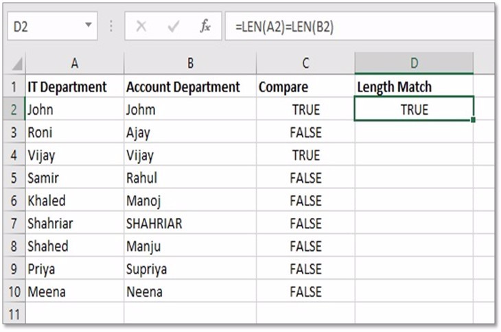
Step 2: Now we can see that the result is showing True for cell A2 and B2. A2 contains John and B2 contains Johm. Here both names contain 4 characters, for this, the result is showing TRUE. Now copy the formula into another cell of column D and see the result.

Step 3: After using the formula in another cell we can see that 3 rows are showing the FALSE result in the above picture. Because their length of characters is not the same. Those rows are row 6, row 8 and row 9.
Tip 2: If you want to see Equal instead of TRUE as result and Not Equal instead of FALSE, you can use this formula instead of our previous formula and see the magic:
- =IF(LEN(A2)=LEN(B2), “Equal”, “Not equal”)
So, now we have learned successfully learned two ways to compare two cells’ value!
15 Pivot Tables Tricks for Pros
15 Pivot Table tricks to make your Excel data analysis smarter! 5,600+ downloads.
Most Popular Tricks are #3, #7 & #12

