One of the features of the Power Query is that it allows you to promote the first row as column headers. Let’s take an example where you have the data set as shown below.
Data Analytics Tricks in Power BI – Guidebook
You too can analyze data like a Data Scientist. No coding needed. No statistics needed.
Analyze & Visualize data using Power BI. (23 tricks in one book)
Use First Row As Headers By Power Query
Here, the headers are not meaningful as it is showing the headers as Column1, Column2, Column3 and so on. Therefore, we have to eliminate them and replace them with the first row’s text.
Here is the step by step guide to using the first row as headers by power query in excel.
Step 1: Load the data table in Power Query Editor
First load the data into the Power Query by clicking on
Home tab > New Source button > Excel > OK
It will give you the data table in this form-
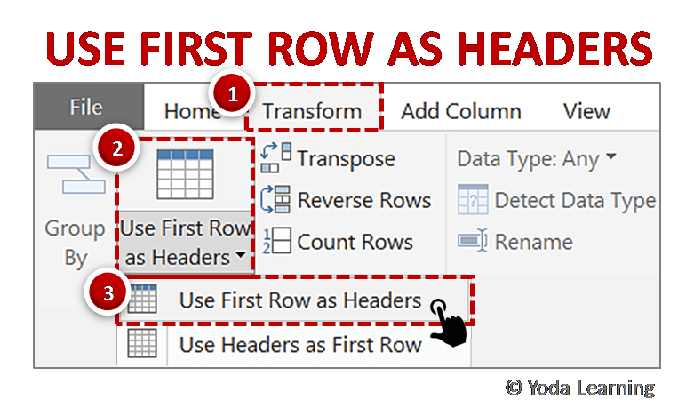
Step 2: To change the auto-generated table headers with the original table headers
Use the ‘Use First Row As Headers’ option.
Go to Transform > Use First Row As Headers option
Note: This option is also available on the ribbon of Home tab in the transform section
Step 3: Close & Apply
Now you get the data table with the new table header and thus you can carry out further operations with your data. Click on ‘Close & Apply’ option to apply the pending changes.
Data Analytics Tricks in Power BI – Guidebook
You too can analyze data like a Data Scientist. No coding needed. No statistics needed.
Analyze & Visualize data using Power BI. (23 tricks in one book)