Sorting data in alphabetical order is helpful when you have large amounts of data in a Pivot Table. Sorting lets you organize the data so it’s easier to find the items you want to analyze.
You can sort a Pivot Table in Excel horizontally or vertically. This allows you to see, at a glance, the rows or columns containing the greatest or the smallest values.
The easiest way to sort a Pivot Table is to select a cell in the row or column that you want to order by and then select either Sort Ascending or Sort Descending, which are represented by the following symbols in the Excel menu:
15 Pivot Tables Tricks for Pros
15 Pivot Table tricks to make your Excel data analysis smarter! 5,600+ downloads.
Most Popular Tricks are #3, #7 & #12
Sort Pivot table
Tips 1: When you sort data, be aware that:
Ø Sort orders vary by locale setting. Make sure that you have the proper locale setting in Regional Settings or Regional and Language Options in Control Panel on your computer.
Ø Data that has leading spaces will affect the sort results. For optimal results, remove any leading spaces before you sort the data.
Ø You can’t sort case-sensitive text entries.
Ø You can’t sort data by a specific format, like cell or font color, or by conditional formatting indicators, such as icon sets.
Now let’s go through the following steps to learn how to sort in in Pivot Table!
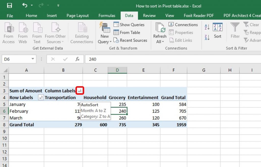
Step 1: In this example, we have a Pivot table that we want to sort in Ascending or Descending order. See the above Picture.
15Excel Data Cleaning Tricks Guidebook
Bored of downloading text heavy / copy-pasted eBooks? If Yes, you will enjoy this guidebook (43 pages)
This table is showing monthly expenses based on some categories like Transport, Entertainment, etc. We will be ascending the category. Categories are decorated in the row serially as Transportation, Household, Grocery, and Entertainment. We will sort these in ascending order. In Column, Label click on the AutoSort button.
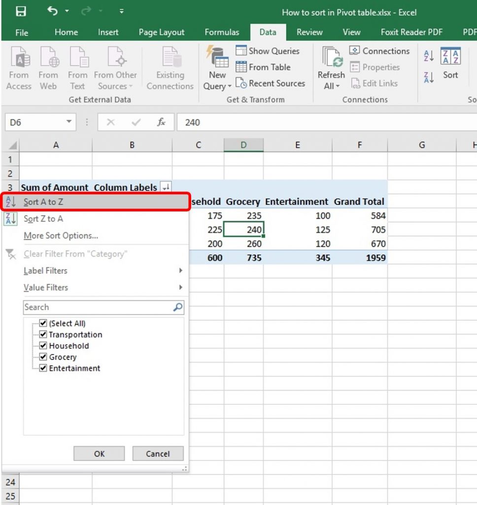
Step 2: Now click Sort A to Z.
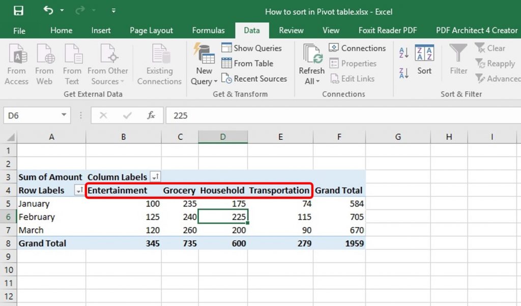
Step 3: After doing that the categories are decorated now as ascending order as like the above picture.
Excel Vlookup formula – Guidebook
Bored of downloading text heavy / copy-pasted eBooks?
If Yes, you will enjoy this guidebook on ‘Excel Vlookup Formulas’ – VLOOKUP, HLOOKUP, MATCH & INDEX.
Step 4: Now let change Month as descending order on the left side column. Click AutoSort button of Row Labels. And click Sort Z to A.
Step 5: Now the month is organized in Descending order as like the above picture.
Step 6: Now let sort in the cost row from a small amount to largest amount. Click on cell B5 which contains 120. Now Click on the Data tab and click Sort from Sort and Filter group.
Step 7: Sort by value Dialog box will appear. Check Smallest to Largest and Left to Right. Click OK.
Step 8: Now the cost is arranged in ascending way as like the above picture.
Conclusion: Sort in the pivot table is possible from A-Z Ascending & Z-A Descending Order.
15 Pivot Tables Tricks for Pros
15 Pivot Table tricks to make your Excel data analysis smarter! 5,600+ downloads.