This example describes how to create a calendar in Excel. The calendar is an important part of keeping all your activities, appointments, meetings, and events organized. You can do a lot with a calendar. People use them as a timesheet to make a work or school schedule to track a project and much more.
There are a couple of different options to make a monthly or yearly calendar. You can create one from scratch using Excel, but that can be a time-consuming, manual task. You can also use a pre-built template of calendar in Excel, with the calendar already formatted for you. There a variety of pre-built calendar templates for Excel, ranging from 12-month calendars, monthly calendars, weekday displays, and calendars with notes.
Excel Vlookup formula – Guidebook

Bored of downloading text heavy / copy-pasted eBooks?
If Yes, you will enjoy this guidebook on ‘Excel Vlookup Formulas’ – VLOOKUP, HLOOKUP, MATCH & INDEX.
How to Create Calendar in Excel 2020
to create Calendar in Excel you should follow the below steps,
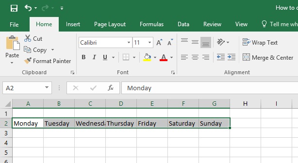
Step 1: Leave the first row in your spreadsheet blank. On the second row type the days of the week (one day per cell). In our example, we typed Monday in cell A2, then Tuesday in cell B2, and typed another day into the rest of this row the same as like above picture.
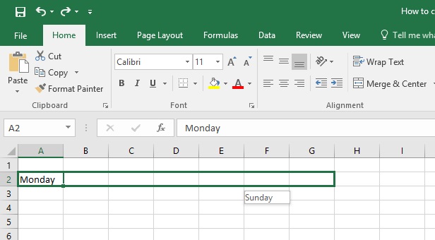
Tips 1: Just type Monday in cell A2 then use the fill handle of the selected cell to drag on the right side of this cell. It will automatically create Tuesday to Sunday in this same row as like the above picture.
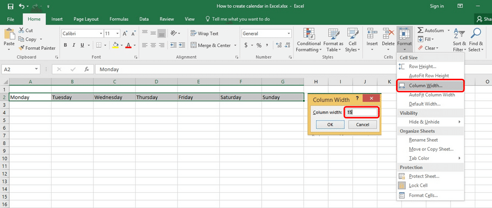
Step 2: To format the weekday headers with ensure proper spacing, highlight the weekdays you just typed and click on Home tab, in the Cells group click Format. Select Column Width and set the width to around 15, depending on how wide you want the calendar.
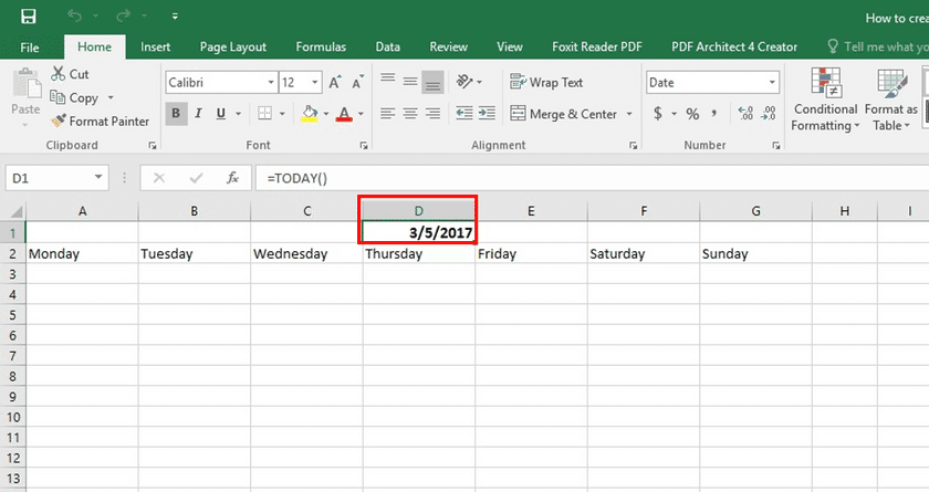
Step 3: In the first blank row 1, we want to add the current month as the Title of the calendar using a formula. Click any cell in the first row and in the fx field above the blank row, type this formula:
=TODAY()
This formula used to tells Excel to show us today’s date in that field. After that, the title of this calendar will be looked like 3/5/2017. But we need the Title as Month only.

Excel Vlookup formula – Guidebook

Bored of downloading text heavy / copy-pasted eBooks?
If Yes, you will enjoy this guidebook on ‘Excel Vlookup Formulas’ – VLOOKUP, HLOOKUP, MATCH & INDEX.
Step 4: Click the cell D1 with the date. Click the Home tab, in the Number group, click the Date drop-down. Select More Number Formats to choose the format you would like for the month title.

Step 5: Now Format Cells dialog box appears. Select Date format from type list. Click OK.
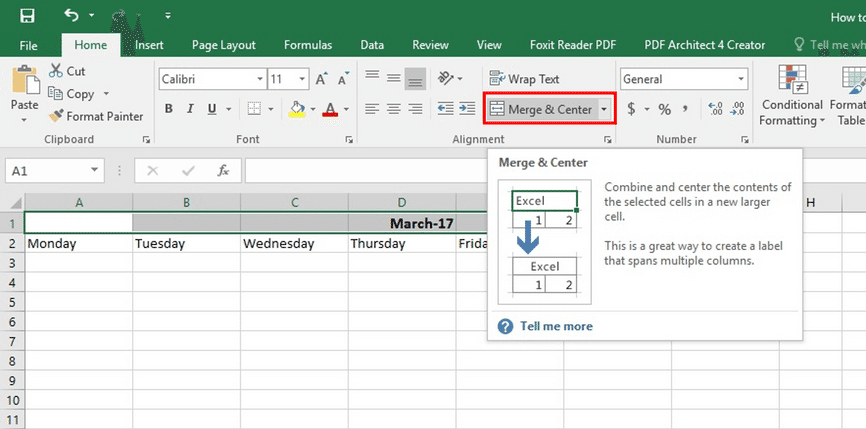
Step 6: Now we have got our Month title with exact format. Select range A1 to G1, Click Home tab, and from the Alignment group click Merge and Center.

Step 7: Now Our month Title is looked like the above picture (March-17).

Step 8: Now we will create the body of our Calendar. We will use borders to create the date boxes. First, highlight your whole spreadsheet. Now, click the paint bucket icon on the Home tab and select white. Your spreadsheet should now have a white background.

Step 9: Highlight five cells under Monday. Click Borders icon in the Home tab and select the outside borders option to outline the first date box in the row.
15 Excel Data Cleaning Tricks Guidebook
Bored of downloading text heavy / copy-pasted eBooks? If Yes, you will enjoy this guidebook (43 pages)

Step 10: Now copy and paste it under the other weekday headers. This duplicates your box for the other days in the week. Do this for five total rows in your sheet as like the above picture.

Step 11: Add borders around the weekday headers and highlight the row with the weekdays. click the borders icon, and choose the All borders.

Step 12: We have created the framework for the calendar, now it’s time to add the dates. Here’s how: For each row in the calendar, enter the first two dates of that week in the first cells in each box. For example, the 1st of this month March of 2017 is Wednesday, enter 1 into the first Wednesday box, and 2 in the Thursday box.
Now hold down Shift and highlight both cells with the numbers. See the above picture. Drag the bottom right corner of the highlighted cells to auto-fill the rest of the week. You must manually enter the first two dates for each row before you can drag and auto-fill the rest of the week. Repeat this for the whole month.

Step 13: Now our Monthly calendar is completed Successfully.

Step 14: Now let’s Decorate Our calendar by coloring. Select Monday to Saturday and Fill the color with your choice. Now fill the color of Sunday as Red, because it is the weekend.

Step 15: Now Select days under Sunday to change font color as Red as like Above picture. Now our Calendar of Month March-2017 is completed successfully. Now you can add notes also on each date if you want like a meeting, schedule, etc.
Step 16: Now copy this month from this Sheet1 to other sheets to create another 12 months. Now our calendar is created successfully.
By this process, you can create a calendar in Excel with a different style
15 Pivot Tables Tricks for Pros
15 Pivot Table tricks to make your Excel data analysis smarter! 5,600+ downloads.
Most Popular Tricks are #3, #7 & #12

