Let’s say you have a worksheet with thousands of rows of data. It would be extremely difficult to see patterns and trends just from examining the raw information. Similar to charts and sparklines, conditional formatting provides another way to visualize data and make worksheets easier to understand.
Excel Vlookup formula – Guidebook

Bored of downloading text heavy / copy-pasted eBooks?
If Yes, you will enjoy this guidebook on ‘Excel Vlookup Formulas’ – VLOOKUP, HLOOKUP, MATCH & INDEX.
Best features of conditional formatting in excel which if coupled with drop down data validation list gives you wonderful reports.
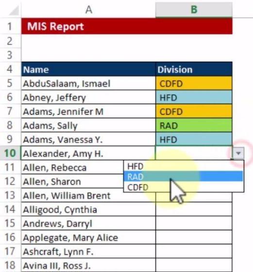
Let me show you an example: In this case, I want to allow divisions to these particular newly joined employees. Whenever I want to select a drop down value which says HFD, it should then get colored according to the predefined color allocation. So if I choose RAD, there you go its green. If I choose RAD once again, again green. If I choose CDFD, orange.

Let’s create Conditional Formatting in Excel with Drop Down List

1. I go to Data. Data validation.

2. I click on Data validation. within which I will have to choose a list

3. And within that, we have the ability to choose the source.

4. So all these cells now contain predefined list values, HFD, RAD, and CDFD.

5. Now choose the entire region where we are supposed to give the division name.
6. Now got to home tab -> Conditional formatting -> new rule. The second option, it says format only cells that contain. So if any of the cell values is equal to yes, if any one of the cell values is equal to, now one option is you can write the hard-coded data, HFD.

Excel Vlookup formula – Guidebook

Bored of downloading text heavy / copy-pasted eBooks?
If Yes, you will enjoy this guidebook on ‘Excel Vlookup Formulas’ – VLOOKUP, HLOOKUP, MATCH & INDEX.
7. Also, you can also choose the cell containing HFD. So this is already fixed, which means whatever you do, wherever you apply this conditional Formatting, this $E$4 indicates this will not move.

So if it’s HFD what color you want to give. I go to format, I go to fill. I put a light blue, ok. Ok,

Now just to test whether it’s working I put HFD. I put RAD, no color. Why no color? Because I have not applied the rule for RAD and CDFD. Create Drop Down List in Excel


So once again I choose the entire block. I go to conditional formatting -> new rule within which I go to the same second option. And this time I say cell value equal to equal to what, equal to the cell containing the value RAD. Let me quickly apply the format. Format which should be light green, perfect. Ok, there you go green.

Once again for the CDFD, I go to Conditional Formatting -> New rule, second option, cell value equal to equal to the cell containing the CDFD value. Let me go to format and choose orange.

So now I choose CDFD, HFD and RAD, all with colors. Create Drop Down List in Excel, So this is how you can link a cell’s excel conditional formatting with another cell so that the value defines the color.

I hope you like our Excel Conditional Formatting Blog, do share with your friend and colleague.
15 Pivot Tables Tricks for Pros
15 Pivot Table tricks to make your Excel data analysis smarter! 5,600+ downloads.
Most Popular Tricks are #3, #7 & #12

