This article is been written to find calculate the ratio in Excel
Ratio: In simple mathematics, relationship or comparison between two more numbers is known as ratios. Ratios are normally written as “:” to show the connection between two numbers, for instance. You can learn such an advanced excel tutorial in our advanced excel dashboard course.
If there are 2 red balls and 3 blue balls on the table you could write their ratio as [2:3]. Unfortunately, there is no systematic way to calculate a ratio, but there is an easy way around for doing the same, you can try the below guidelines to calculate the ratio in Excel.
Excel Vlookup formula – Guidebook
Bored of downloading text heavy / copy-pasted eBooks?
If Yes, you will enjoy this guidebook on ‘Excel Vlookup Formulas’ – VLOOKUP, HLOOKUP, MATCH & INDEX.
Method 1: How to Calculate the Ratio in Excel.
Calculate Ratio Formula: To calculate the Ratio in excel, the Shop 1 will be divided by GCD and the Shop 2 will be divided by GCD. You can place a colon between those two numbers. Example: To see the ratio, enter this formula in cell E2 = B2/GCD(B2,C2)&”:”&C2/GCD(B2,C2).
Calculate the Ratio of Products between Two Shops
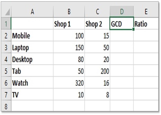
Step 1: Create a table the same as the above picture. This table is showing a number of products in the store of two shops. We are going to calculate the ratio of each product between these 2 shops. Column D is for calculating GCD and Column E is for a ratio.
What is GCD?
The GCD Function is used to calculate the greatest common denominator between two or more values. We can use GCD to then create our ratios. The GCD Function is extremely easy to use. Simply type =GCD( followed by the numbers that you wish to find the greatest common divisor of (separated by commas).
Formula: =GCD(Number 1, Number 2)
Once you understand how GCD works you can use the function to find your ratios by dividing each of the two numbers by their GCD and separating the answers with a colon “:”. Hence, now we are ready on how to calculate a ratio.
First, we need to calculate GCD in column D then we will calculate the ratio in column E using GCD.
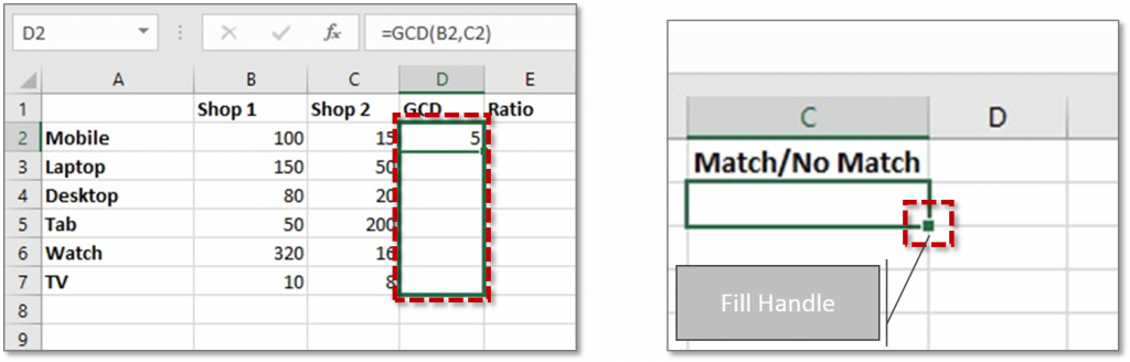
Step 2: In cell D2 type this formula to calculate GCD between B2 and C2. =GCD(B2,C2)
Step 3: Now we have got GCD result 5 for cell B2 and C2. So, now copy this formula into other cells of the column using Fill Handle dragging below to other cells of column D.
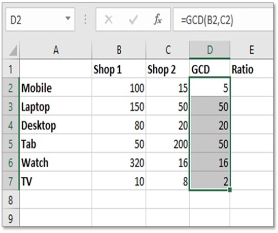
Step 4: Now we have got all GCD values of all rows in column D. Now let’s Calculate ratio.
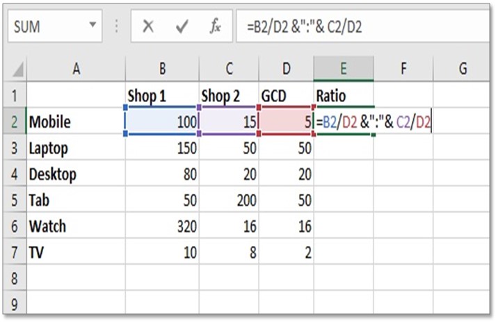
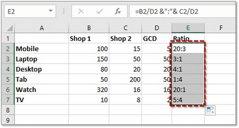
Step 5: In a cell, E2 type this formula to calculate ratio:
=B2/D2 &”:”& C2/D2
Press ENTER. Now we have got the ratio between 100 and 15 as 20:3 in cell E2.
Step 6: Copy the ratio formula in another cell of column E. Finally, we have got the ratio of the whole table. So, we have successfully learned how to calculate the ratio in excel.
15 Pivot Tables Tricks for Pros
15 Pivot Table tricks to make your Excel data analysis smarter! 5,600+ downloads.
Most Popular Tricks are #3, #7 & #12
Method 2: Create the Ratio Formula using Text Function
Another method of calculating Ratio using TEXT and SUBSTITUTE – these work in all versions of Excel.
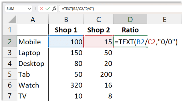
Step 1: To calculate the ratio for each cell
Enter this formula in cell D2 cell =TEXT(B2/C2,”0/0″)
The result will be 20/3.
Note: To practice with us. We have shared the Excel sheet. You can download it from the link below
When it is useful? Most of the time the most annoying problem is when the data is taken from ERP or other…
1 Comment
Comments are closed.
peterprism
There are many formulae which we can use for a different purpose and you can visit the ms excel customer support number to know about the different formulae to calculate the ratio.


There are many formulae which we can use for a different purpose and you can visit the ms excel customer support number to know about the different formulae to calculate the ratio.