Struggling with profit and loss? Or still, figuring out how to calculate the profit margin in excel? Here is your answer, the Profit margin is an important figure for business because it tells the percentage of each profited sale. Profit margins are important when pricing products, pursuing financing and generating sales reports.
If you create the spreadsheet and input the formula properly, Microsoft Excel will calculate profit margins. If you need to calculate a profit margin, you can easily do so with a simple formula that uses the sale price and the cost. Knowing how to calculate your profit margin will help you take control of your business and ensure that each sale nets the profit you expect.
Excel Vlookup formula – Guidebook
Bored of downloading text heavy / copy-pasted eBooks?
If Yes, you will enjoy this guidebook on ‘Excel Vlookup Formulas’ – VLOOKUP, HLOOKUP, MATCH & INDEX.
Method 1: What is Profit Margin in Excel, here’s the simple step?
Profit Margin Formula in Excel is an input formula in the final column the profit margin on sale will be calculated. The Excel Profit Margin Formula is the amount of profit divided by the amount of the sale or (C2/A2)100 to get value in percentage. Example: Profit Margin Formula in Excel calculation (120/200)100 to produce a 60 percent profit margin result.
Also to calculate profit percentage in excel, type profit percentage formula of Excel i.e. (A2-B2) into C2 the profit cell. Once you calculate the profit percentage in D2 Cell, drag the corner of the cell to get the rest of the profit percentage of sale data.
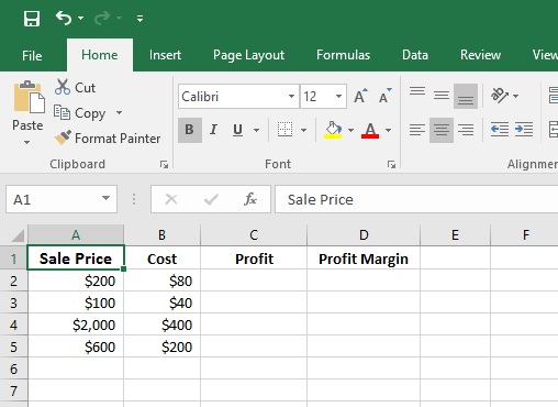
Step 1: Create a table the same as like given picture. This table is showing Sale price in column A, Cost in column B, Profit in column C and Profit Margin in column D.
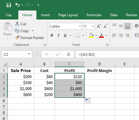
Step 2: Before we calculate profit margin formula, we need to calculate the profit by input a formula in the cells of column C. the formula would be like this in cell C2:
=(A2-B2) The formula should read “=(A2-B2)” to subtract the cost of the product from the sale price. The difference is your overall profit, in this example, the formula result would be $120. Then press ENTER.
Step 3: Now you will get the profit value in cell C2. Now do the same for another cell of column C. after that the table will be looked like the above picture.
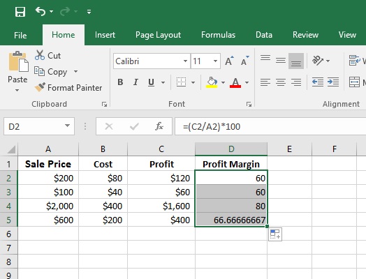
Step 4: Now we will calculate the profit Margin in column D using this formula in cell D2:
=(C2/A2)*100 This formula will calculate the percentage value of Profit margin. Now, Press ENTER. Do the same for another cell of column D. You will get all profit margin for each Sale.
15 Pivot Tables Tricks for Pros
15 Pivot Table tricks to make your Excel data analysis smarter! 5,600+ downloads.
Most Popular Tricks are #3, #7 & #12
Method 2: Calculate YoY Percentage Change in Excel
Sometimes you may have monthly or yearly data and you want to calculate Year over Year % Growth to make dashboard in Excel, the percent change calculation is very often used. You can do that easily.
This article will show you how to calculate Year over Year percentage growth in Excel.
But before we go any further, let’s take a closer look of Raw Data
The Excel sheet is about [Sales] and [Profit] earned each year from 2017 to 2023. There are four columns, [Year], [Sales], [Profit] and YoY Growth %. We will calculate the percentage growth year over year in Column D.
Note: We have shared the Excel sheet. You can download it from the link below